🧠 Key takeaways
Cell type deconvolution method allows us to gain single-cell resolution information out of the old bulk samples.
Follow the four rules of thumb when performing cell type deconvolution.
Practically, when performing cell type deconvolution, run more than one method, check whether they agree, and validate against any measured proportions you have (for example, blood counts or histology).
⚙️ Environment setup
Install conda:
Before creating the environment, ensure that conda is installed on your system.
Save the yml content:
Copy the content from the yml tab into a file named
environment.yml.
Create the environment:
Open a terminal or command prompt.
Run the following command:
conda env create -f environment.yml
Activate the environment:
After the environment is created, activate it using:
conda activate <environment_name>Replace
<environment_name>with the name specified in theenvironment.ymlfile. In the yml file it will look like this:name: <environment_name>
Verify the installation:
Check that the environment was created successfully by running:
conda env list
name: bulk-deconvolution
channels:
  - conda-forge
dependencies:
  - conda-forge::ipykernel=7.3.0
  - conda-forge::ipywidgets=8.1.9
  - conda-forge::python=3.12.16
  - pip
  - pip:
      - lamindb==2.12.2
      # rectanglepy pins numpy<2 and scipy==1.13.0, which has no wheels for Python 3.13
      - rectanglepy==1.7.0
      # pyarrow 26 requires numpy>=2
      - pyarrow==25.0.0
      - scanpy==1.11.5
      - seaborn==0.13.2
Introduction
Imagine tasting a fruit smoothie and trying to work out how much banana, strawberry and mango went into it. You can’t see the individual pieces anymore, everything has been blended into one average flavor. But if you know what each fruit tastes like on its own, you can make a good guess at the recipe.
Bulk RNA-seq is the smoothie. A tissue sample contains many different cell types, and sequencing it in bulk blends all their transcripts into one average expression profile. Information about which cells contributed what is lost, which creates a real interpretation problem. Let’s say a gene goes up in diseased tissue compared to healthy tissue. Two very different things could explain that Shen-Orr & Gaujoux, 2013:
each cell is expressing more of the gene, or
the cells that express the gene have become more common.
From the bulk profile alone, you can’t tell these apart. Cell type deconvolution recovers the recipe. Given a bulk expression profile and a description of what each cell type “tastes like” (its typical expression profile, the reference), deconvolution estimates how much each cell type contributes to the sample Cobos et al., 2021.
Why not just use single-cell data?
You may start thinking: “We’ve been talking about single-cell analysis the whole time, why are we going back to bulk now?” Although single-cell RNA-seq measures cell types directly, the bulk data already exists, and there is a lot of it. Bulk RNA-seq is cheaper, easier to run in clinical settings, and decades of cohorts, biobanks and patient archives were profiled this way Cobos et al., 2023. Deconvolution lets you reuse a relatively small single-cell dataset as a reference to read cell composition out of thousands of bulk samples you could never afford to re-profile at single-cell resolution.
Single-cell data has also changed deconvolution itself. Reference profiles used to come from physically sorted cell populations, which covered only the cell types someone thought to sort for, and only those with good antibodies Monaco et al., 2019Aran et al., 2017. Single-cell atlases now provide references for many tissues, organisms and conditions without that pre-selection Aliee & Theis, 2021Newman et al., 2019.
What makes it hard
The smoothie picture also shows where deconvolution breaks:
A missing ingredient. If the smoothie contains kiwi but your list of fruits doesn’t, its flavour gets wrongly attributed to whatever fruits are on the list. A cell type absent from the reference distorts every other estimate Cobos et al., 2021Jin & Liu, 2021.
Strong flavours dominate. A small amount of a strong-tasting fruit can outweigh a lot of a mild one. Likewise, cells differ in how much RNA they contain, so the estimated contribution to the RNA is not the same as the fraction of cells Monaco et al., 2019.
These caveats are the reason for the practical recommendations that follow.
What makes deconvolution work: four rules of thumb
Going back to the smoothie: the quality of your recipe guess depends less on how clever you are and more on what you know about the fruit. The same holds for deconvolution. A large benchmark that systematically varied each step of the pipeline found that the choices that matter most are not the method itself but how the data and reference are prepared: keeping data on a linear scale, using a reference that covers every cell type in the mixture, and choosing marker genes sensibly Cobos et al., 2021. We restate these findings as four rules of thumb:
Include every cell type present in the sample in the reference.
Use a resolution at which cell types are actually distinguishable.
Keep the data in linear scale, and don’t rescale it.
Choose marker genes carefully.
Four rules of thumb for deconvolution based on Cobos et al., 2021
1. Include every cell type present in the sample in the reference
If an ingredient is missing from your list, its flavour does not disappear: it gets blamed on whatever fruits are on the list. Leaving a cell type out of the reference that is present in the bulk sample made results substantially worse, no matter which method, transformation or normalization was used. When you cannot be sure your reference is complete, prefer methods that explicitly estimate an “unknown” or “other” fraction (see the method table below).
2. Use a resolution at which cell types are actually distinguishable
Banana and strawberry are easy to tell apart in a smoothie; two kinds of raspberry are not. Closely related cell types share most of their expression, so estimates for one leak into the other. Benchmarks observe exactly this: signal is wrongly assigned to cell types that are absent from a mixture, likely because related cell types share signatures or because their marker genes are not specific enough. More recent benchmarks likewise find that accuracy depends on how similar the cell types in the reference are Dietrich et al., 2026. In practice, start with broad cell types (T cells, B cells, monocytes) and only split them further if the finer types have clearly distinct expression.
3. Keep the data in linear scale, and don’t rescale it
Mixing is additive: if a sample is 30% T cells and 70% monocytes, the T cells contribute 30% of the transcripts. That additivity only holds for counts (or count-like values), not for log-transformed data, where adding two values no longer corresponds to mixing two samples. Keeping the data in linear scale consistently gave the lowest errors, while log and variance-stabilizing transformations gave two- to four-fold higher median errors.
The same logic applies to scaling. Rescaling genes or samples into a fixed range (0 to 1, or z-scores) throws away the actual amounts that deconvolution relies on, like setting every smoothie’s strongest flavour to “maximum”. In the benchmark, these scalings and quantile normalization performed poorly, while standard library-size normalizations mattered little for most methods.
4. Choose marker genes carefully
Not every fruit is useful for telling a recipe apart: water content tastes the same in all of them. Genes expressed at similar levels in every cell type carry no information about composition and only add noise. Marker selection was one of the three most influential factors for classical (non-single-cell) deconvolution methods. A useful marker is not just high in its own cell type; it is clearly higher than in the runner-up, the cell type with the second-highest expression. The benchmark recommends a stringent selection built on exactly this comparison, in line with earlier findings that markers work best when expressed mainly in one cell type Hunt et al., 2018 and when genes with a small fold change between the top two cell types are removed Monaco et al., 2019. Within such a marker set, using all markers worked best, and picking only a handful per cell type (e.g. the top two) could be worse than random for some methods. Good marker genes are high in one cell type and low in the others; feature-selection tools such as AutoGeneS pick genes that make cell types as distinguishable as possible Aliee & Theis, 2021.
What the benchmarks say
Deconvolution methods have been compared many times, on immune cells Sturm et al., 2019, on pseudo-bulk mixtures built from single-cell data Cobos et al., 2021, under varied simulation settings Jin & Liu, 2021, in tumours Tran et al., 2023, on paired bulk and single-cell data Cobos et al., 2023, and across transcriptomic and methylation data Amblard et al., 2025.
A few lessons hold across them:
No method wins everywhere. The most recent large benchmark of single-cell-informed methods found substantial differences in accuracy, scalability and robustness that depended on cell-type similarity, reference composition and where the data came from Dietrich et al., 2026.
Single-cell references are competitive. Methods that use scRNA-seq references performed comparably to the best classical methods, while semi-supervised approaches had higher errors Cobos et al., 2021.
Fine-grained types are where methods diverge. In breast tumours, most methods mistook normal epithelial cells for cancer cells as tumour purity rose; BayesPrism and DWLS made the fewest false calls and did best on granular immune lineages Tran et al., 2023.
The reference matters as much as the method. Profiling bulk and single-cell data from the same samples improved both single-cell preprocessing and deconvolution accuracy Cobos et al., 2023.
The practical takeaway: run more than one method, check whether they agree, and validate against any measured proportions you have (for example, blood counts or histology).
Method families
Most methods differ in how they turn the reference and the bulk profile into proportions. The table groups them by that idea; expand each family for details and examples.
| Family | Core idea (smoothie version) | Needs a full reference? | Output | Examples |
|---|---|---|---|---|
| Regression | Find the mix of reference fruits whose blend tastes closest to the smoothie | Yes | Proportions | CIBERSORTx, MuSiC, DWLS, FARDEEP, Bisque, SCDC |
| Enrichment / marker scores | Score how strongly each fruit’s signature flavour comes through, one fruit at a time | Marker lists only | Scores (not always proportions) | xCell, MCP-counter |
| Bayesian | Treat each fruit’s taste as uncertain and infer the most probable recipe, plus how each fruit tasted in this smoothie | Yes (used as a prior) | Proportions + per-cell-type expression | BayesPrism |
| Deep learning | Train a model on thousands of smoothies with known recipes, then predict | Yes (to simulate training data) | Proportions | Scaden |
| Reference-free | Recover both the ingredients and the recipe from many smoothies at once | No | Proportions + inferred profiles | Linseed |
Methods-Citations
Here are the citations for the examples in the table above:
Regression:
CIBERSORTx Newman et al., 2019}
MuSiC Wang et al., 2019}
DWLS Tsoucas et al., 2019}
FARDEEP Hao et al., 2019}
Bisque Jew et al., 2020}
SCDC Dong et al., 2020}
dtangle Hunt et al., 2018}
SQUID Cobos et al., 2023}
Enrichment / marker scores:
xCell Aran et al., 2017}
MCP-counter Becht et al., 2016}
Bayesian:
BayesPrism Chu et al., 2022
Deep learning:
Scaden Menden et al., 2020}
Reference-free:
Linseed Zaitsev et al., 2019}
Strengths and weaknesses of method families
| Family | Strengths | Weaknesses |
|---|---|---|
| Regression | Interpretable and fast | Sensitive to missing cell types and to highly similar cell types |
| Enrichment / marker scores | Robust; need only marker lists | Scores are not proportions; accuracy drops when many related cell types are scored |
| Bayesian | Can model uncertainty and per-cell-type expression | Slower and more complex |
| Deep learning | Can learn complex relationships | Needs a lot of training data; may not generalize well |
| Reference-free | No reference needed | Needs many samples; components must be labelled as cell types afterwards |
Among the many available deconvolution tools, we use Rectangle Eder et al., 2026 to demonstrate a use case. Rectangle is a Python framework from the scverse ecosystem that learns cell-type signatures directly from an annotated single-cell reference.
The output is a samples × cell types table of estimated proportions, with an additional Unknown column.
Deconvolving bulk COVID-19 whole blood samples
In the following use case we deconvolve 49 bulk whole blood RNA-seq samples from 39 patients with COVID-19 and 10 healthy controls Aschenbrenner et al., 2020 using Rectangle Eder et al., 2026. As single-cell reference, we use whole blood scRNA-seq data of patients with COVID-19 and controls Schulte-Schrepping et al., 2020. For most of the patients, neutrophil and lymphocyte counts were measured in the clinic, which lets us check the estimates against an independent measurement.
Environment setup
import lamindb as ln
import matplotlib.pyplot as plt
import pandas as pd
import rectanglepy as rectangle
import scanpy as sc
import seaborn as sns
from scipy import stats

ln.connect("theislab/sc-best-practices")

ln.track("HsJRsKmLcB2Q")
Output
→ connected lamindb: theislab/sc-best-practices
! It looks like you are running jupyter lab but don't have jupyter-server module installed. Please install it via pip install jupyter-server
→ loaded Transform('HsJRsKmLcB2Q0002', key='bulk_deconvolution.ipynb'), started new Run('8POULixJNZAVUB4P') at 2026-11-09 12:26:05 UTC
Loading the data
All three datasets are stored in the lamindb instance of this book. The bulk expression is already converted to TPM, with one row per sample and one column per gene, which is the layout Rectangle expects.
bulks = ln.Artifact.get(
    key="deconvolution/bulk_deconvolution/covid19_wholeblood_bulk_tpm.parquet"
).load()
metadata = ln.Artifact.get(
    key="deconvolution/bulk_deconvolution/covid19_wholeblood_metadata.parquet"
).load()
bulks.iloc[:5, :5]The metadata tells us whether a sample comes from a patient or a healthy control, together with the measured blood counts.
metadata[
    ["status", "Total.neutrophil.count...mm3.", "Total.lymphocyte.count...mm3."]
].head()adata = ln.Artifact.get(
key="deconvolution/bulk_deconvolution/schulte_schrepping2020_covid19_wholeblood_counts.h5ad"
).load()
adataAnnData object with n_obs × n_vars = 89883 × 33417
obs: 'orig.ident', 'nCount_RNA', 'nFeature_RNA', 'nCount_HTO', 'nFeature_HTO', 'percent.mito', 'percent.hb', 'HTO_maxID', 'HTO_secondID', 'HTO_margin', 'HTO_classification', 'HTO_classification.global', 'hash.ID', 'demultID', 'donor', 'onset_of_symptoms', 'days_after_onset', 'sampleID', 'date_of_sampling', 'experiment', 'cartridge', 'platform', 'purification', 'cells', 'age', 'sex', 'group_per_sample', 'who_per_sample', 'disease_stage', 'diagnosis', 'oxygen', 'outcome', 'comorbidities', 'COVID.19.related_medication_and_anti.microbials', 'primary_complaint', 'RNA_snn_res.0.8', 'cluster_labels_res.0.8', 'new.order', 'hpca.labels', 'blueprint.labels', 'monaco.labels', 'immune.labels', 'dmap.labels', 'hemato.labels'
obsm: 'X_umap'Preparing the single-cell reference
The study profiled both fresh whole blood and peripheral blood mononuclear cells (PBMCs).
PBMC isolation removes granulocytes such as neutrophils, which make up most of the white blood cells in whole blood.
Since our bulk samples are whole blood, the reference only contains the whole blood cells, so that it covers every cell type in the mixture (rule 1).
adata.X holds the unnormalized counts that Rectangle expects.
adata.obs["cluster_labels_res.0.8"].value_counts()cluster_labels_res.0.8
Neutrophils_1 22714
Neutrophils_2 18675
Neutrophils_3 9986
CD4_T_cells_1 6278
CD14_Monocytes_1 5362
Neutrophils_4 4710
CD8_T_cells 3255
Megakaryocytes 3180
NK_cells 2916
B_cells_1 2561
CD4_T_cells_2 1917
Mixed_cells 1727
Immature Neutrophils_1 1317
CD16_Monocytes 983
Immature Neutrophils_2 981
CD14_Monocytes_3 632
Eosinophils 579
CD14_Monocytes_2 556
CD4_T_cells_3 409
Plasmablast 390
Prol. cells 247
mDC 235
B_cells_2 138
pDC 86
CD34+ GATA2+ cells 49
Name: count, dtype: int64Quality control has already been performed by the authors, so we skip it here.
We remove two clusters that do not represent a single cell type: Mixed_cells, which express markers of several cell types and are likely doublets, and dividing cells (Prol. cells), which are grouped by their cell-cycle genes rather than their identity.
Rectangle builds one expression profile per cell type, and these clusters would blend the profiles of others.
The authors annotated the data at a fine resolution: there are four neutrophil clusters, three CD4⁺ T cell clusters and three CD14⁺ monocyte clusters. These clusters are states of the same cell type and differ in only a few genes, which is too little to tell them apart in a bulk profile (rule 2). We therefore merge the clusters of each cell type into a single label.
cell_types = {
    "Neutrophils_1": "Neutrophils",
    "Neutrophils_2": "Neutrophils",
    "Neutrophils_3": "Neutrophils",
    "Neutrophils_4": "Neutrophils",
    "Immature Neutrophils_1": "Immature neutrophils",
    "Immature Neutrophils_2": "Immature neutrophils",
    "Eosinophils": "Eosinophils",
    "CD14_Monocytes_1": "CD14 monocytes",
    "CD14_Monocytes_2": "CD14 monocytes",
    "CD14_Monocytes_3": "CD14 monocytes",
    "CD16_Monocytes": "CD16 monocytes",
    "mDC": "mDCs",
    "pDC": "pDCs",
    "CD4_T_cells_1": "CD4 T cells",
    "CD4_T_cells_2": "CD4 T cells",
    "CD4_T_cells_3": "CD4 T cells",
    "CD8_T_cells": "CD8 T cells",
    "NK_cells": "NK cells",
    "B_cells_1": "B cells",
    "B_cells_2": "B cells",
    "Plasmablast": "Plasmablasts",
    "Megakaryocytes": "Megakaryocytes",
    "CD34+ GATA2+ cells": "CD34+ GATA2+ cells",
}

adata = adata[adata.obs["cluster_labels_res.0.8"].isin(cell_types)].copy()
adata.obs["cell_type"] = (
    adata.obs["cluster_labels_res.0.8"].map(cell_types).astype("category")
)
adata.obs["cell_type"].value_counts()
cell_type
Neutrophils 56085
CD4 T cells 8604
CD14 monocytes 6550
CD8 T cells 3255
Megakaryocytes 3180
NK cells 2916
B cells 2699
Immature neutrophils 2298
CD16 monocytes 983
Eosinophils 579
Plasmablasts 390
mDCs 235
pDCs 86
CD34+ GATA2+ cells 49
Name: count, dtype: int64The authors also computed a UMAP embedding, which we use to look at the cell types in the reference.
sc.pl.umap(adata, color="cell_type")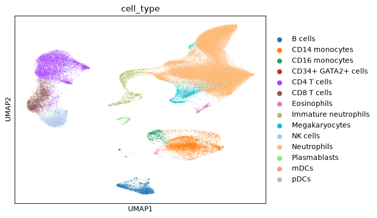
Running Rectangle
A single call to rectangle.rectangle builds the reference and deconvolves all bulk samples.
Under the hood, it:
sums the counts of all cells of a cell type into a pseudobulk profile, the cell type’s “taste”,
selects marker genes by differential expression between the cell types, and tunes the cutoffs on simulated mixtures with known proportions (rule 4),
groups similar cell types into clusters, deconvolves the clusters first and then the cell types within them, which helps with closely related cell types (rule 2),
corrects for the different amounts of RNA per cell, so that the output are fractions of cells and not of RNA,
estimates how much of each bulk sample is not explained by the reference and reports it as
Unknown(rule 1).
Rectangle uses only the genes measured in both datasets. Selecting marker genes is the slow part and takes a while on a reference of this size.
fractions, signatures = rectangle.rectangle(adata, bulks, cell_type_col="cell_type")Output
2026-11-09 13:26:15.419 | INFO | rectanglepy.pp.create_signature:build_rectangle_signatures:355 - Using 21225 common genes between bulks and single-cell data
2026-11-09 13:26:18.432 | INFO | rectanglepy.pp.create_signature:_de_analysis:209 - Starting DE analysis
2026-11-09 13:26:19.052 | INFO | rectanglepy.pp.create_signature:_run_deseq2:152 - Running DE analysis for B cells
2026-11-09 13:26:21.029 | INFO | rectanglepy.pp.create_signature:_run_deseq2:152 - Running DE analysis for CD14 monocytes
2026-11-09 13:26:22.173 | INFO | rectanglepy.pp.create_signature:_run_deseq2:152 - Running DE analysis for CD16 monocytes
2026-11-09 13:26:23.529 | INFO | rectanglepy.pp.create_signature:_run_deseq2:152 - Running DE analysis for CD34+ GATA2+ cells
2026-11-09 13:26:24.846 | INFO | rectanglepy.pp.create_signature:_run_deseq2:152 - Running DE analysis for CD4 T cells
2026-11-09 13:26:25.412 | INFO | rectanglepy.pp.create_signature:_run_deseq2:152 - Running DE analysis for CD8 T cells
2026-11-09 13:26:25.924 | INFO | rectanglepy.pp.create_signature:_run_deseq2:152 - Running DE analysis for Eosinophils
2026-11-09 13:26:26.326 | INFO | rectanglepy.pp.create_signature:_run_deseq2:152 - Running DE analysis for Immature neutrophils
2026-11-09 13:26:27.302 | INFO | rectanglepy.pp.create_signature:_run_deseq2:152 - Running DE analysis for Megakaryocytes
2026-11-09 13:26:27.842 | INFO | rectanglepy.pp.create_signature:_run_deseq2:152 - Running DE analysis for NK cells
2026-11-09 13:26:28.864 | INFO | rectanglepy.pp.create_signature:_run_deseq2:152 - Running DE analysis for Neutrophils
2026-11-09 13:26:29.533 | INFO | rectanglepy.pp.create_signature:_run_deseq2:152 - Running DE analysis for Plasmablasts
2026-11-09 13:26:31.012 | INFO | rectanglepy.pp.create_signature:_run_deseq2:152 - Running DE analysis for mDCs
2026-11-09 13:26:32.269 | INFO | rectanglepy.pp.create_signature:_run_deseq2:152 - Running DE analysis for pDCs
2026-11-09 13:26:33.303 | INFO | rectanglepy.pp.create_signature:_de_analysis:222 - Optimizing cutoff parameters p and lfc
2026-11-09 13:26:33.304 | INFO | rectanglepy.pp.create_signature:_optimize_parameters:452 - generating pseudo bulks
2026-11-09 13:26:34.138 | INFO | rectanglepy.pp.create_signature:_get_marker_genes:249 - Optimal condition number: 79
2026-11-09 13:26:34.375 | INFO | rectanglepy.pp.create_signature:_optimize_parameters:460 - RMSE:0.05406091372887245, Pearson R:0.5968690432441663 for p=0.05, lfc=1.6
Polishing not needed - no active set detected at optimal point
Polishing not needed - no active set detected at optimal point
Polishing not needed - no active set detected at optimal point
Polishing not needed - no active set detected at optimal point
Polishing not needed - no active set detected at optimal point
Polishing not needed - no active set detected at optimal point
Polishing not needed - no active set detected at optimal point
2026-11-09 13:26:34.471 | INFO | rectanglepy.pp.create_signature:_get_marker_genes:249 - Optimal condition number: 79
2026-11-09 13:26:34.635 | INFO | rectanglepy.pp.create_signature:_optimize_parameters:460 - RMSE:0.05440664121676341, Pearson R:0.593202627041872 for p=0.05, lfc=1.7
Polishing not needed - no active set detected at optimal point
Polishing not needed - no active set detected at optimal point
Polishing not needed - no active set detected at optimal point
Polishing not needed - no active set detected at optimal point
Polishing not needed - no active set detected at optimal point
Polishing not needed - no active set detected at optimal point
Polishing not needed - no active set detected at optimal point
2026-11-09 13:26:34.730 | INFO | rectanglepy.pp.create_signature:_get_marker_genes:249 - Optimal condition number: 79
2026-11-09 13:26:34.919 | INFO | rectanglepy.pp.create_signature:_optimize_parameters:460 - RMSE:0.056120497151173586, Pearson R:0.5769065545993959 for p=0.05, lfc=1.8
2026-11-09 13:26:35.005 | INFO | rectanglepy.pp.create_signature:_get_marker_genes:249 - Optimal condition number: 79
Polishing not needed - no active set detected at optimal point
Polishing not needed - no active set detected at optimal point
Polishing not needed - no active set detected at optimal point
2026-11-09 13:26:35.178 | INFO | rectanglepy.pp.create_signature:_optimize_parameters:460 - RMSE:0.05678676856075405, Pearson R:0.5726782733365512 for p=0.05, lfc=1.9
Polishing not needed - no active set detected at optimal point
Polishing not needed - no active set detected at optimal point
Polishing not needed - no active set detected at optimal point
2026-11-09 13:26:35.264 | INFO | rectanglepy.pp.create_signature:_get_marker_genes:249 - Optimal condition number: 79
2026-11-09 13:26:35.431 | INFO | rectanglepy.pp.create_signature:_optimize_parameters:460 - RMSE:0.05714272415313951, Pearson R:0.5706805335400458 for p=0.05, lfc=2.0
2026-11-09 13:26:35.512 | INFO | rectanglepy.pp.create_signature:_get_marker_genes:249 - Optimal condition number: 76
Polishing not needed - no active set detected at optimal point
Polishing not needed - no active set detected at optimal point
Polishing not needed - no active set detected at optimal point
2026-11-09 13:26:35.670 | INFO | rectanglepy.pp.create_signature:_optimize_parameters:460 - RMSE:0.057210635135514415, Pearson R:0.5681991517678615 for p=0.05, lfc=2.1
2026-11-09 13:26:35.747 | INFO | rectanglepy.pp.create_signature:_get_marker_genes:249 - Optimal condition number: 69
Polishing not needed - no active set detected at optimal point
Polishing not needed - no active set detected at optimal point
2026-11-09 13:26:35.912 | INFO | rectanglepy.pp.create_signature:_optimize_parameters:460 - RMSE:0.05727311944715092, Pearson R:0.5679043273384133 for p=0.05, lfc=2.2
2026-11-09 13:26:35.913 | INFO     | rectanglepy.pp.create_signature:_de_analysis:232 - Optimization done
 Best cutoffs  p: 0.05 and lfc: 1.6
Polishing not needed - no active set detected at optimal point
Polishing not needed - no active set detected at optimal point
2026-11-09 13:26:36.007 | INFO | rectanglepy.pp.create_signature:_get_marker_genes:249 - Optimal condition number: 79
2026-11-09 13:26:36.009 | INFO | rectanglepy.pp.create_signature:build_rectangle_signatures:385 - Starting rectangle cluster analysis
2026-11-09 13:26:36.024 | INFO | rectanglepy.pp.create_signature:_create_clustered_data:290 - Starting clustered analysis
2026-11-09 13:26:36.664 | INFO | rectanglepy.pp.create_signature:_de_analysis:209 - Starting DE analysis
2026-11-09 13:26:37.375 | INFO | rectanglepy.pp.create_signature:_run_deseq2:152 - Running DE analysis for 1
2026-11-09 13:26:37.976 | INFO | rectanglepy.pp.create_signature:_run_deseq2:152 - Running DE analysis for 4
2026-11-09 13:26:39.034 | INFO | rectanglepy.pp.create_signature:_run_deseq2:152 - Running DE analysis for 6
2026-11-09 13:26:39.533 | INFO | rectanglepy.pp.create_signature:_run_deseq2:152 - Running DE analysis for B cells
2026-11-09 13:26:40.052 | INFO | rectanglepy.pp.create_signature:_run_deseq2:152 - Running DE analysis for CD34+ GATA2+ cells
2026-11-09 13:26:41.277 | INFO | rectanglepy.pp.create_signature:_run_deseq2:152 - Running DE analysis for Eosinophils
2026-11-09 13:26:41.691 | INFO | rectanglepy.pp.create_signature:_run_deseq2:152 - Running DE analysis for Immature neutrophils
2026-11-09 13:26:42.588 | INFO | rectanglepy.pp.create_signature:_run_deseq2:152 - Running DE analysis for Plasmablasts
2026-11-09 13:26:43.981 | INFO | rectanglepy.pp.create_signature:_run_deseq2:152 - Running DE analysis for mDCs
2026-11-09 13:26:45.113 | INFO | rectanglepy.pp.create_signature:_run_deseq2:152 - Running DE analysis for pDCs
2026-11-09 13:26:46.170 | INFO | rectanglepy.pp.create_signature:_get_marker_genes:249 - Optimal condition number: 68
2026-11-09 13:26:46.390 | INFO     | rectanglepy.tl.deconvolution:_process_bulk:442 - Deconvolute fractions for bulk: 0
2026-11-09 13:26:46.390 | INFO     | rectanglepy.tl.deconvolution:_process_bulk:442 - Deconvolute fractions for bulk: 4
2026-11-09 13:26:46.390 | INFO     | rectanglepy.tl.deconvolution:_process_bulk:442 - Deconvolute fractions for bulk: 1
2026-11-09 13:26:46.390 | INFO     | rectanglepy.tl.deconvolution:_process_bulk:442 - Deconvolute fractions for bulk: 3
2026-11-09 13:26:46.394 | INFO     | rectanglepy.tl.deconvolution:_process_bulk:442 - Deconvolute fractions for bulk: 6
2026-11-09 13:26:46.395 | INFO     | rectanglepy.tl.deconvolution:_process_bulk:442 - Deconvolute fractions for bulk: 7
2026-11-09 13:26:46.395 | INFO     | rectanglepy.tl.deconvolution:_process_bulk:442 - Deconvolute fractions for bulk: 5
2026-11-09 13:26:46.398 | INFO     | rectanglepy.tl.deconvolution:_process_bulk:442 - Deconvolute fractions for bulk: 2
2026-11-09 13:26:47.212 | INFO     | rectanglepy.tl.deconvolution:_process_bulk:450 - Finished deconvolution for bulk: 3
2026-11-09 13:26:47.217 | INFO     | rectanglepy.tl.deconvolution:_process_bulk:450 - Finished deconvolution for bulk: 1
2026-11-09 13:26:47.223 | INFO     | rectanglepy.tl.deconvolution:_process_bulk:442 - Deconvolute fractions for bulk: 8
2026-11-09 13:26:47.246 | INFO     | rectanglepy.tl.deconvolution:_process_bulk:442 - Deconvolute fractions for bulk: 9
2026-11-09 13:26:47.262 | INFO     | rectanglepy.tl.deconvolution:_process_bulk:450 - Finished deconvolution for bulk: 4
2026-11-09 13:26:47.266 | INFO     | rectanglepy.tl.deconvolution:_process_bulk:450 - Finished deconvolution for bulk: 0
2026-11-09 13:26:47.273 | INFO     | rectanglepy.tl.deconvolution:_process_bulk:442 - Deconvolute fractions for bulk: 10
2026-11-09 13:26:47.280 | INFO     | rectanglepy.tl.deconvolution:_process_bulk:442 - Deconvolute fractions for bulk: 11
2026-11-09 13:26:48.047 | INFO     | rectanglepy.tl.deconvolution:_process_bulk:450 - Finished deconvolution for bulk: 8
2026-11-09 13:26:48.057 | INFO     | rectanglepy.tl.deconvolution:_process_bulk:450 - Finished deconvolution for bulk: 10
2026-11-09 13:26:48.060 | INFO     | rectanglepy.tl.deconvolution:_process_bulk:442 - Deconvolute fractions for bulk: 12
2026-11-09 13:26:48.074 | INFO     | rectanglepy.tl.deconvolution:_process_bulk:442 - Deconvolute fractions for bulk: 13
2026-11-09 13:26:48.109 | INFO     | rectanglepy.tl.deconvolution:_process_bulk:450 - Finished deconvolution for bulk: 11
2026-11-09 13:26:48.121 | INFO     | rectanglepy.tl.deconvolution:_process_bulk:442 - Deconvolute fractions for bulk: 14
2026-11-09 13:26:48.130 | INFO     | rectanglepy.tl.deconvolution:_process_bulk:450 - Finished deconvolution for bulk: 9
2026-11-09 13:26:48.143 | INFO     | rectanglepy.tl.deconvolution:_process_bulk:442 - Deconvolute fractions for bulk: 15
2026-11-09 13:26:48.166 | INFO     | rectanglepy.tl.deconvolution:_process_bulk:450 - Finished deconvolution for bulk: 5
2026-11-09 13:26:48.189 | INFO     | rectanglepy.tl.deconvolution:_process_bulk:442 - Deconvolute fractions for bulk: 16
2026-11-09 13:26:48.255 | INFO     | rectanglepy.tl.deconvolution:_process_bulk:450 - Finished deconvolution for bulk: 7
2026-11-09 13:26:48.279 | INFO     | rectanglepy.tl.deconvolution:_process_bulk:442 - Deconvolute fractions for bulk: 17
2026-11-09 13:26:48.309 | INFO     | rectanglepy.tl.deconvolution:_process_bulk:450 - Finished deconvolution for bulk: 6
2026-11-09 13:26:48.336 | INFO     | rectanglepy.tl.deconvolution:_process_bulk:442 - Deconvolute fractions for bulk: 18
2026-11-09 13:26:48.427 | INFO     | rectanglepy.tl.deconvolution:_process_bulk:450 - Finished deconvolution for bulk: 2
2026-11-09 13:26:48.457 | INFO | rectanglepy.tl.deconvolution:_process_bulk:442 - Deconvolute fractions for bulk: 19
2026-11-09 13:26:48.805 | INFO     | rectanglepy.tl.deconvolution:_process_bulk:450 - Finished deconvolution for bulk: 12
2026-11-09 13:26:48.817 | INFO     | rectanglepy.tl.deconvolution:_process_bulk:442 - Deconvolute fractions for bulk: 20
2026-11-09 13:26:48.875 | INFO     | rectanglepy.tl.deconvolution:_process_bulk:450 - Finished deconvolution for bulk: 13
2026-11-09 13:26:48.889 | INFO     | rectanglepy.tl.deconvolution:_process_bulk:442 - Deconvolute fractions for bulk: 21
2026-11-09 13:26:48.941 | INFO     | rectanglepy.tl.deconvolution:_process_bulk:450 - Finished deconvolution for bulk: 14
2026-11-09 13:26:48.964 | INFO     | rectanglepy.tl.deconvolution:_process_bulk:442 - Deconvolute fractions for bulk: 22
2026-11-09 13:26:49.122 | INFO     | rectanglepy.tl.deconvolution:_process_bulk:450 - Finished deconvolution for bulk: 15
2026-11-09 13:26:49.165 | INFO     | rectanglepy.tl.deconvolution:_process_bulk:442 - Deconvolute fractions for bulk: 23
2026-11-09 13:26:49.566 | INFO     | rectanglepy.tl.deconvolution:_process_bulk:450 - Finished deconvolution for bulk: 20
2026-11-09 13:26:49.577 | INFO     | rectanglepy.tl.deconvolution:_process_bulk:442 - Deconvolute fractions for bulk: 24
2026-11-09 13:26:49.635 | INFO     | rectanglepy.tl.deconvolution:_process_bulk:450 - Finished deconvolution for bulk: 19
2026-11-09 13:26:49.636 | INFO     | rectanglepy.tl.deconvolution:_process_bulk:450 - Finished deconvolution for bulk: 21
2026-11-09 13:26:49.645 | INFO     | rectanglepy.tl.deconvolution:_process_bulk:442 - Deconvolute fractions for bulk: 25
2026-11-09 13:26:49.659 | INFO     | rectanglepy.tl.deconvolution:_process_bulk:442 - Deconvolute fractions for bulk: 26
2026-11-09 13:26:50.026 | INFO     | rectanglepy.tl.deconvolution:_process_bulk:450 - Finished deconvolution for bulk: 23
2026-11-09 13:26:50.035 | INFO     | rectanglepy.tl.deconvolution:_process_bulk:442 - Deconvolute fractions for bulk: 27
2026-11-09 13:26:50.114 | INFO     | rectanglepy.tl.deconvolution:_process_bulk:450 - Finished deconvolution for bulk: 17
2026-11-09 13:26:50.137 | INFO     | rectanglepy.tl.deconvolution:_process_bulk:442 - Deconvolute fractions for bulk: 28
2026-11-09 13:26:50.200 | INFO     | rectanglepy.tl.deconvolution:_process_bulk:450 - Finished deconvolution for bulk: 18
2026-11-09 13:26:50.230 | INFO     | rectanglepy.tl.deconvolution:_process_bulk:442 - Deconvolute fractions for bulk: 29
2026-11-09 13:26:50.238 | INFO     | rectanglepy.tl.deconvolution:_process_bulk:450 - Finished deconvolution for bulk: 16
2026-11-09 13:26:50.266 | INFO     | rectanglepy.tl.deconvolution:_process_bulk:442 - Deconvolute fractions for bulk: 30
2026-11-09 13:26:50.303 | INFO     | rectanglepy.tl.deconvolution:_process_bulk:450 - Finished deconvolution for bulk: 24
2026-11-09 13:26:50.311 | INFO     | rectanglepy.tl.deconvolution:_process_bulk:442 - Deconvolute fractions for bulk: 31
2026-11-09 13:26:50.358 | INFO     | rectanglepy.tl.deconvolution:_process_bulk:450 - Finished deconvolution for bulk: 25
2026-11-09 13:26:50.368 | INFO     | rectanglepy.tl.deconvolution:_process_bulk:442 - Deconvolute fractions for bulk: 32
2026-11-09 13:26:50.486 | INFO     | rectanglepy.tl.deconvolution:_process_bulk:450 - Finished deconvolution for bulk: 26
2026-11-09 13:26:50.503 | INFO     | rectanglepy.tl.deconvolution:_process_bulk:442 - Deconvolute fractions for bulk: 33
2026-11-09 13:26:50.672 | INFO     | rectanglepy.tl.deconvolution:_process_bulk:450 - Finished deconvolution for bulk: 22
2026-11-09 13:26:50.702 | INFO     | rectanglepy.tl.deconvolution:_process_bulk:442 - Deconvolute fractions for bulk: 34
2026-11-09 13:26:50.852 | INFO     | rectanglepy.tl.deconvolution:_process_bulk:450 - Finished deconvolution for bulk: 27
2026-11-09 13:26:50.864 | INFO     | rectanglepy.tl.deconvolution:_process_bulk:442 - Deconvolute fractions for bulk: 35
2026-11-09 13:26:51.027 | INFO     | rectanglepy.tl.deconvolution:_process_bulk:450 - Finished deconvolution for bulk: 31
2026-11-09 13:26:51.040 | INFO     | rectanglepy.tl.deconvolution:_process_bulk:442 - Deconvolute fractions for bulk: 36
2026-11-09 13:26:51.168 | INFO     | rectanglepy.tl.deconvolution:_process_bulk:450 - Finished deconvolution for bulk: 32
2026-11-09 13:26:51.179 | INFO     | rectanglepy.tl.deconvolution:_process_bulk:442 - Deconvolute fractions for bulk: 37
2026-11-09 13:26:51.349 | INFO     | rectanglepy.tl.deconvolution:_process_bulk:450 - Finished deconvolution for bulk: 33
2026-11-09 13:26:51.356 | INFO     | rectanglepy.tl.deconvolution:_process_bulk:442 - Deconvolute fractions for bulk: 38
2026-11-09 13:26:51.637 | INFO     | rectanglepy.tl.deconvolution:_process_bulk:450 - Finished deconvolution for bulk: 35
2026-11-09 13:26:51.651 | INFO     | rectanglepy.tl.deconvolution:_process_bulk:442 - Deconvolute fractions for bulk: 39
2026-11-09 13:26:51.778 | INFO     | rectanglepy.tl.deconvolution:_process_bulk:450 - Finished deconvolution for bulk: 28
2026-11-09 13:26:51.805 | INFO     | rectanglepy.tl.deconvolution:_process_bulk:450 - Finished deconvolution for bulk: 29
2026-11-09 13:26:51.807 | INFO     | rectanglepy.tl.deconvolution:_process_bulk:442 - Deconvolute fractions for bulk: 40
2026-11-09 13:26:51.828 | INFO     | rectanglepy.tl.deconvolution:_process_bulk:450 - Finished deconvolution for bulk: 36
2026-11-09 13:26:51.832 | INFO     | rectanglepy.tl.deconvolution:_process_bulk:442 - Deconvolute fractions for bulk: 41
2026-11-09 13:26:51.871 | INFO     | rectanglepy.tl.deconvolution:_process_bulk:442 - Deconvolute fractions for bulk: 42
2026-11-09 13:26:51.960 | INFO     | rectanglepy.tl.deconvolution:_process_bulk:450 - Finished deconvolution for bulk: 30
2026-11-09 13:26:51.990 | INFO     | rectanglepy.tl.deconvolution:_process_bulk:442 - Deconvolute fractions for bulk: 43
2026-11-09 13:26:52.216 | INFO     | rectanglepy.tl.deconvolution:_process_bulk:450 - Finished deconvolution for bulk: 38
2026-11-09 13:26:52.224 | INFO     | rectanglepy.tl.deconvolution:_process_bulk:442 - Deconvolute fractions for bulk: 44
2026-11-09 13:26:52.428 | INFO     | rectanglepy.tl.deconvolution:_process_bulk:450 - Finished deconvolution for bulk: 39
2026-11-09 13:26:52.440 | INFO     | rectanglepy.tl.deconvolution:_process_bulk:450 - Finished deconvolution for bulk: 34
2026-11-09 13:26:52.443 | INFO     | rectanglepy.tl.deconvolution:_process_bulk:442 - Deconvolute fractions for bulk: 45
2026-11-09 13:26:52.474 | INFO     | rectanglepy.tl.deconvolution:_process_bulk:442 - Deconvolute fractions for bulk: 46
2026-11-09 13:26:52.482 | INFO     | rectanglepy.tl.deconvolution:_process_bulk:450 - Finished deconvolution for bulk: 37
2026-11-09 13:26:52.506 | INFO     | rectanglepy.tl.deconvolution:_process_bulk:442 - Deconvolute fractions for bulk: 47
2026-11-09 13:26:52.571 | INFO     | rectanglepy.tl.deconvolution:_process_bulk:450 - Finished deconvolution for bulk: 41
2026-11-09 13:26:52.580 | INFO     | rectanglepy.tl.deconvolution:_process_bulk:442 - Deconvolute fractions for bulk: 48
2026-11-09 13:26:52.606 | INFO     | rectanglepy.tl.deconvolution:_process_bulk:450 - Finished deconvolution for bulk: 40
2026-11-09 13:26:53.022 | INFO | rectanglepy.tl.deconvolution:_process_bulk:450 - Finished deconvolution for bulk: 44
2026-11-09 13:26:53.289 | INFO     | rectanglepy.tl.deconvolution:_process_bulk:450 - Finished deconvolution for bulk: 45
2026-11-09 13:26:53.365 | INFO     | rectanglepy.tl.deconvolution:_process_bulk:450 - Finished deconvolution for bulk: 47
2026-11-09 13:26:53.391 | INFO     | rectanglepy.tl.deconvolution:_process_bulk:450 - Finished deconvolution for bulk: 48
2026-11-09 13:26:53.454 | INFO     | rectanglepy.tl.deconvolution:_process_bulk:450 - Finished deconvolution for bulk: 42
2026-11-09 13:26:53.482 | INFO     | rectanglepy.tl.deconvolution:_process_bulk:450 - Finished deconvolution for bulk: 43
2026-11-09 13:26:53.502 | INFO | rectanglepy.tl.deconvolution:_process_bulk:450 - Finished deconvolution for bulk: 46
The returned signatures summarizes the reference that Rectangle built, including how many marker genes it selected per cell type and which cell types it grouped together.
signaturesRectangleSignatureResult
──────────────────────────────────────────────────
Total Signature genes: 466
Cell types: 14
B cells marker genes: ['AFF3', 'BANK1', 'BIRC3', 'CD22', 'CD37', 'CD79A', 'CD79B', 'FCMR', 'FCRL1', 'HLA-DOB', 'HVCN1', 'IGHD', 'IKZF3', 'LINC00926', 'MEF2C', 'MS4A1', 'PAX5', 'PLPP5', 'RALGPS2', 'TNFRSF13C']
CD14 monocytes marker genes: ['APLP2', 'CCR1', 'CD14', 'CD163', 'CD300E', 'CD33', 'CD36', 'CD68', 'CD93', 'CPVL', 'CSTA', 'CTSB', 'CTSS', 'CYP1B1', 'DUSP6', 'FCN1', 'KCTD12', 'LGALS3', 'LRP1', 'MAFB', 'MS4A6A', 'PLBD1', 'SLC7A7', 'TMEM176A', 'TMEM176B', 'VCAN', 'ZNF385A']
CD16 monocytes marker genes: ['ABI3', 'ADGRE1', 'AIF1', 'CD300E', 'CD68', 'CD86', 'CDKN1C', 'COTL1', 'CSF1R', 'CTSL', 'CUX1', 'CXCL16', 'FAM110A', 'FCGR3A', 'HMOX1', 'IER5', 'INSIG1', 'KDM1B', 'KLF4', 'LILRA1', 'LILRB1', 'LILRB2', 'LRRC25', 'LST1', 'MAFB', 'MS4A4A', 'MS4A7', 'MTSS1', 'NAAA', 'NAGA', 'NR4A1', 'PECAM1', 'PLXNB2', 'POU2F2', 'RHOC', 'RRAS', 'SCIMP', 'SIDT2', 'SIGLEC10', 'SLC31A2', 'SLC7A7', 'SMIM25', 'TCF7L2', 'TIMP1', 'TMEM176B', 'TNFRSF1B']
CD34+ GATA2+ cells marker genes: ['AMD1', 'ANKRD28', 'ATF7IP2', 'BAALC', 'BEX3', 'BLMH', 'BZW2', 'CCNG1', 'CD34', 'CDK6', 'DKC1', 'EBPL', 'FAM117A', 'FAM30A', 'FAM98B', 'FHL1', 'FSCN1', 'GAS5', 'HMGA1', 'HNRNPA1', 'HSP90AB1', 'HSPB1', 'IGFBP7', 'IL18', 'IL1B', 'IMPDH2', 'ISYNA1', 'JUP', 'LAPTM4B', 'MAP7', 'MSI2', 'MSRB3', 'MTURN', 'MYB', 'NME4', 'NPR3', 'NREP', 'NRIP1', 'PRKACB', 'REC8', 'SMIM24', 'SNHG19', 'SNHG7', 'SNHG8', 'SOX4', 'SPINK2', 'STMN1', 'TARBP1', 'TESPA1', 'TFRC', 'TGFBRAP1', 'TM7SF3', 'TSC22D1', 'YBX3']
CD4 T cells marker genes: ['AC245427.1', 'BCL11B', 'CD2', 'CD3D', 'CD3E', 'CD3G', 'DGKA', 'ETS1', 'GIMAP7', 'IL32', 'IL7R', 'ITK', 'LEF1', 'LTB', 'MAL', 'PCED1B-AS1', 'RCAN3', 'SPOCK2', 'TCF7', 'TRAC', 'TRBC2']
CD8 T cells marker genes: ['AC245427.1', 'ARL4C', 'BCL11B', 'CCL5', 'CD2', 'CD3D', 'CD3E', 'CD3G', 'CD8A', 'CTSW', 'FGFBP2', 'GIMAP7', 'GZMA', 'GZMH', 'IKZF3', 'IL32', 'IL7R', 'KLRD1', 'LCK', 'NKG7', 'PRF1', 'PRKCH', 'RASGRP1', 'RUNX3', 'SLFN12L', 'SPOCK2', 'TRAC', 'TRBC2', 'TRGC2']
Eosinophils marker genes: ['CAMK1D', 'CLC', 'CSF2RB', 'SSH2', 'TBXAS1']
Immature neutrophils marker genes: ['ABCA13', 'AL034397.3', 'ALDH3B1', 'AMPD3', 'ANXA3', 'APMAP', 'ARG1', 'ATP8B4', 'AZU1', 'B4GALT5', 'BPI', 'BST1', 'C20orf27', 'CAMP', 'CD24', 'CD63', 'CDA', 'CDCA7L', 'CEACAM1', 'CEACAM6', 'CEACAM8', 'CHI3L1', 'CHIT1', 'CITED4', 'CKAP4', 'CLEC4D', 'CLEC5A', 'COL17A1', 'CPNE2', 'CPNE3', 'CRISP3', 'CSGALNACT1', 'CTSD', 'CYBB', 'CYP4F3', 'CYSTM1', 'DEFA3', 'DEFA4', 'EMB', 'ERG', 'FAR2', 'FBXO9', 'GADD45A', 'GBE1', 'GCA', 'GPI', 'GPR160', 'GSN', 'GYG1', 'GYS1', 'HK3', 'HMGB2', 'HMGN2', 'HP', 'INHBA', 'IRAK3', 'ITGAM', 'JDP2', 'LCN2', 'LIN7A', 'LTF', 'MBOAT2', 'MCEMP1', 'MCU', 'MFSD10', 'MMP8', 'MS4A3', 'MSRA', 'NLRC4', 'OLFM4', 'OLR1', 'OSCAR', 'PADI4', 'PDE4D', 'PGD', 'PGLYRP1', 'PLBD1', 'PRAM1', 'PYGL']
Megakaryocytes marker genes: ['FCGR3B', 'NRGN', 'PF4', 'PPBP', 'SPARC', 'STEAP4']
NK cells marker genes: ['ADGRG1', 'ARL4C', 'CCL4', 'CCL5', 'CD247', 'CD7', 'CST7', 'CTSW', 'CX3CR1', 'FGFBP2', 'GNLY', 'GZMA', 'GZMB', 'GZMH', 'HOPX', 'IL2RB', 'KLRB1', 'KLRD1', 'KLRF1', 'NKG7', 'PRF1', 'PRKCH', 'PYHIN1', 'RUNX3', 'SH2D1B', 'SLFN12L', 'SLFN5', 'SPON2', 'TRDC']
Neutrophils marker genes: ['ALPL', 'CMTM2', 'FCGR3B', 'G0S2', 'IFIT2', 'IFIT3', 'PROK2']
Plasmablasts marker genes: ['AC012236.1', 'ALG5', 'AQP3', 'B4GALT3', 'CALR', 'CALU', 'CAV1', 'CCNC', 'CCND2', 'CD27', 'CD38', 'CEP128', 'CLIC4', 'CLPTM1L', 'CPNE5', 'CRELD2', 'CYCS', 'DANCR', 'DDOST', 'DENND5B', 'DERL1', 'DERL3', 'DNAJB11', 'EAF2', 'EDEM1', 'ELL2', 'ENAM', 'ERLEC1', 'FCRL5', 'FKBP11', 'FKBP2', 'GGH', 'GLCCI1', 'GMPPA', 'GNL3', 'HDLBP', 'HSP90B1', 'HSPA13', 'HSPA5', 'HYOU1', 'IGHA1', 'IGHG1', 'IGHG2', 'IGHG3', 'IGHGP', 'IGKC', 'IGLC2', 'IGLC3', 'IRF4', 'ISOC2', 'JCHAIN', 'KDELR2', 'LMAN1', 'LMAN2', 'LRRC59', 'MAGED1', 'MAN1A1', 'MANEA', 'MANF', 'MLEC', 'MYBL2', 'MYDGF', 'MYO1D', 'MZB1', 'NME1', 'NT5DC2', 'OSTC', 'P4HB', 'PDIA4', 'PDIA6', 'PIM2', 'PLPP5', 'PNOC', 'POU2AF1', 'PPIB', 'PRDM1', 'PRDX1', 'PRDX4', 'PREB']
mDCs marker genes: ['AHR', 'ANXA2', 'AP1S2', 'CD1C', 'CD33', 'CD86', 'CIITA', 'CLEC10A', 'CLIC2', 'CPVL', 'CST3', 'DPYSL2', 'FCER1A', 'HLA-DMA', 'HLA-DMB', 'HLA-DOA', 'HLA-DPA1', 'HLA-DPB1', 'HLA-DQA1', 'HLA-DQB1', 'HLA-DRA', 'HLA-DRB1', 'HLA-DRB5', 'HLA-DRB6', 'KCTD12', 'LGALS2', 'LY86', 'MS4A6A', 'NAPSB', 'NDRG2', 'PEA15', 'PID1', 'RTN1', 'S100A10', 'SAMHD1', 'SHTN1', 'ZNF385A']
pDCs marker genes: ['AC023590.1', 'APP', 'BCL11A', 'BLNK', 'C12orf75', 'CBFA2T3', 'CCDC50', 'CCDC88A', 'CD4', 'CLEC4C', 'CYB561A3', 'DAB2', 'DCK', 'DERL3', 'DNASE1L3', 'DUSP5', 'FMNL3', 'GAPT', 'GPR183', 'GZMB', 'HERPUD1', 'HIGD1A', 'IDH3A', 'IRF7', 'IRF8', 'ITM2C', 'LILRA4', 'LILRB4', 'MAP1A', 'MAPKAPK2', 'MGST2', 'MIF4GD', 'MPEG1', 'NAPSB', 'NPC1', 'NPC2', 'OFD1', 'OPN3', 'P2RY14', 'PACSIN1', 'PAXX', 'PHB', 'PLAC8', 'PLD4', 'PPP1R14B', 'PTMS', 'PTPRS', 'REPIN1', 'RNASE6', 'RUNX2', 'SCAMP5', 'SEC61B', 'SELENOS', 'SERPINF1', 'SLC15A4', 'SLC7A5', 'SMPD3', 'SPIB', 'SUSD1', 'TCF4', 'TEX14', 'TGFBI', 'TNFRSF21', 'TPM2', 'TSPAN13', 'TSPAN3', 'UGCG', 'UNC93B1', 'VEGFB', 'ZFAT']
Cluster assignments: ['B cells', 4, 4, 'CD34+ GATA2+ cells', 6, 6, 'Eosinophils', 'Immature neutrophils', 1, 6, 1, 'Plasmablasts', 'mDCs', 'pDCs']
Unknown cell content analysis: Yes
DGE Optimization result available:
Best cutoffs: p: 0.05, lfc: 1.6Outputs
The main output of all cell type deconvolution methods is a samples × cell types matrix of estimated proportions.
Each row sums to one, and Rectangle adds the Unknown column for content that the reference does not explain.
fractions.round(3).head()A stacked bar per sample gives an overview of the estimated composition.
order = (
    fractions.mean()
    .sort_values(ascending=False)
    .index.drop("Unknown")
    .append(pd.Index(["Unknown"]))
)
samples = metadata.sort_values("status").index
colors = sns.color_palette("tab20", len(order) - 1) + [(0.8, 0.8, 0.8)]

ax = fractions.loc[samples, order].plot.bar(
    stacked=True, width=0.9, figsize=(12, 4), color=colors
)
n_covid = (metadata["status"] == "covid").sum()
ax.axvline(n_covid - 0.5, color="black")
ax.set_xticks([])
ax.set_xlabel("COVID-19 (left) and healthy (right) samples")
ax.set_ylabel("Estimated fraction")
ax.legend(bbox_to_anchor=(1, 1), loc="upper left", frameon=False)
plt.show()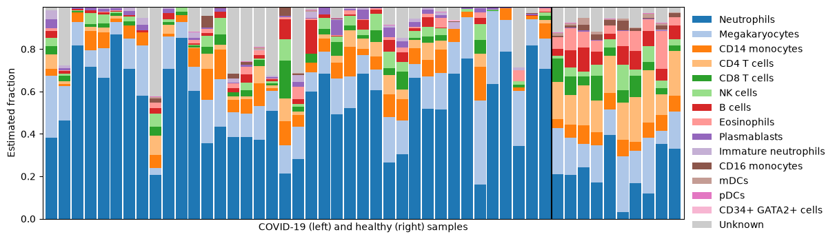
Neutrophils make up the largest part of most patient samples. Two other columns need a closer look.
The Megakaryocytes cluster of the reference mostly captures platelets, fragments of megakaryocytes that circulate in large numbers in the blood.
Platelets far outnumber white blood cells but carry little RNA, so their estimated fraction depends strongly on the correction for RNA content.
Clinical blood counts, in contrast, only cover white blood cells.
The Unknown column is the part of each sample that the reference does not explain.
Whole blood contains cell types that are missing from the single-cell reference, for example red blood cell precursors, which contribute globin transcripts to the bulk RNA.
Without an Unknown column, their expression would be assigned to the cell types in the reference (rule 1).
Validating against blood counts
If the true proportions are known, we can check the estimates against them.
The patients’ neutrophil and lymphocyte counts were measured in the clinic, for the healthy controls they are missing.
The counts are absolute numbers per mm³ of blood, while deconvolution estimates relative fractions, so we compare the share of neutrophils among neutrophils and lymphocytes.
This ratio is also unaffected by platelets and by the Unknown fraction, which the blood counts do not include.
lymphocytes = ["CD4 T cells", "CD8 T cells", "NK cells", "B cells", "Plasmablasts"]
neutrophils = ["Neutrophils", "Immature neutrophils"]

measured = metadata["Total.neutrophil.count...mm3."] / (
    metadata["Total.neutrophil.count...mm3."]
    + metadata["Total.lymphocyte.count...mm3."]
)
estimated = fractions[neutrophils].sum(axis=1) / fractions[
    neutrophils + lymphocytes
].sum(axis=1)

validation = pd.DataFrame({"measured": measured, "estimated": estimated}).dropna()
r, p = stats.pearsonr(validation["measured"], validation["estimated"])
print(f"Pearson r = {r:.2f} (p = {p:.1e}, n = {len(validation)} samples)")

ax = sns.scatterplot(data=validation, x="measured", y="estimated")
ax.axline((0.5, 0.5), slope=1, color="grey", linestyle="--")
ax.set_xlabel("Neutrophil share, blood counts")
ax.set_ylabel("Neutrophil share, Rectangle")
plt.show()
Pearson r = 0.68 (p = 2.2e-05, n = 32 samples)
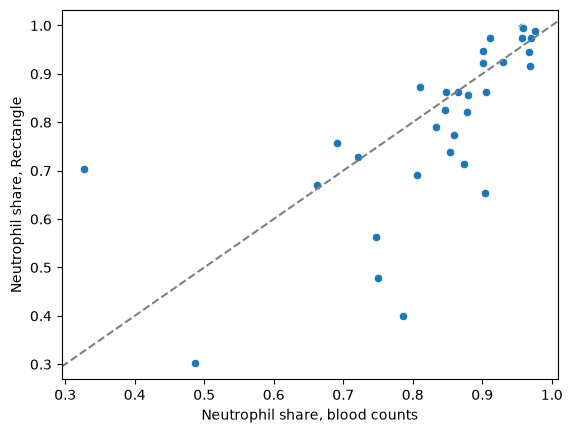
The estimated and measured neutrophil shares agree well, with most samples close to the diagonal. A few samples are off by more than 0.2, so the estimates of individual samples should be interpreted with care.
Comparing COVID-19 patients and healthy controls
We can also look for changes in cell type composition between patients and healthy controls. For each cell type, we compare the estimated fractions with a Mann-Whitney U test and correct the p-values for testing many cell types. Keep in mind that the fractions of a sample sum to one, so an increase in one cell type forces others to decrease. The chapter on compositional analysis explains how to test for changes in composition while taking this into account.
covid = metadata["status"] == "covid"
tests = pd.DataFrame(
    {
        "mean covid": fractions[covid].mean(),
        "mean healthy": fractions[~covid].mean(),
        "p": [
            stats.mannwhitneyu(
                fractions.loc[covid, ct], fractions.loc[~covid, ct]
            ).pvalue
            for ct in fractions.columns
        ],
    }
)
tests["p adj"] = stats.false_discovery_control(tests["p"])
tests.sort_values("p adj").round({"mean covid": 3, "mean healthy": 3})We plot four of the cell types that change significantly between the groups. CD4⁺ T cells and eosinophils have the smallest p-values. Neutrophils show the largest change and are the cell type we validated against the blood counts above. Immature neutrophils increase the most relative to their level in healthy blood. mDCs and CD16 monocytes also change significantly, but we leave them out because they make up less than 2% of the cells, and deconvolution is least reliable for rare cell types Tsoucas et al., 2019.
selected = ["Neutrophils", "Immature neutrophils", "CD4 T cells", "Eosinophils"]
plot_df = (
    fractions[selected]
    .join(metadata["status"])
    .melt(id_vars="status", var_name="cell type", value_name="fraction")
)

g = sns.catplot(
    data=plot_df,
    x="status",
    y="fraction",
    col="cell type",
    kind="box",
    showfliers=False,
    sharey=False,
    height=3,
    aspect=0.8,
)
g.map_dataframe(sns.stripplot, x="status", y="fraction", color="black", size=3)
g.set_titles("{col_name}")
plt.show()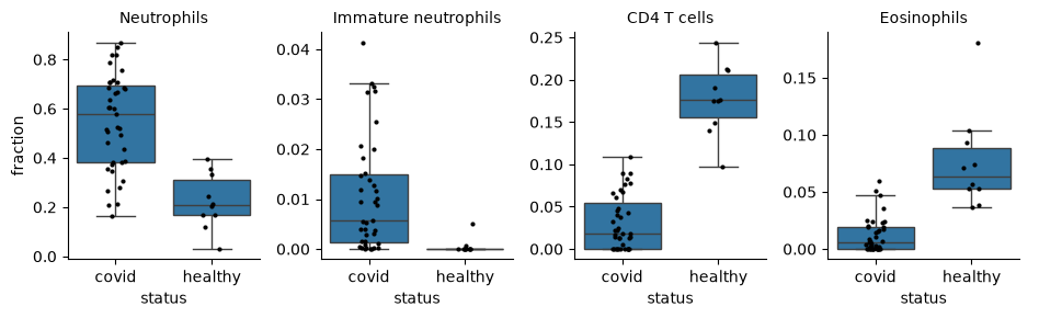
Compared to the healthy controls, the patients have more neutrophils, including immature neutrophils, and fewer CD4⁺ T cells and eosinophils. The table shows the same direction for B cells and CD8⁺ T cells. Immature neutrophils are rare in healthy blood, and the single-cell study also found them in patients with severe COVID-19 Schulte-Schrepping et al., 2020. With 10 controls and fractions that depend on each other, these results describe the cohort rather than establish effects, and a dedicated compositional analysis would be the next step.
ln.finish()Output
! cells [(1, 4), (14, 13)] were not run consecutively
→ to save the notebook html, run: lamin save /home/seokim/seocodes_linux/single-cell-best-practices/jupyter-book/deconvolution/bulk_deconvolution.ipynb
→ finished Run('8POULixJNZAVUB4P') after 52s at 2026-11-09 12:26:58 UTC
→ go to: https://lamin.ai/theislab/sc-best-practices/run/8POULixJNZAVUB4P
→ to update your notebook from the CLI, run: lamin save /home/seokim/seocodes_linux/single-cell-best-practices/jupyter-book/deconvolution/bulk_deconvolution.ipynb
Limitations and traps
The four rules of thumb cover the most common sources of error. Our example of deconvolving bulk COVID-19 whole blood samples shows a few more traps:
Fractions of cells are not fractions of RNA. Converting between the two relies on an estimate of each cell type’s RNA content, so the fractions of cell types with little RNA, such as platelets (
Megakaryocytes), are uncertain.The reference is not the sample. Differences in patients, technology or disease state change gene expression and get attributed to the wrong cell types; a reference from the same samples helps Cobos et al., 2023.
Unknown content is estimated, not identified. The
Unknowncolumn tells you how much of a sample the reference misses, but not which cells Cobos et al., 2021Jin & Liu, 2021.Trust cohort trends more than single samples. A few samples were off by more than 0.2, rare cell types are the least reliable Tsoucas et al., 2019, and fractions are compositional.
New directions
Deconvolution methods are moving beyond cell type proportions:
Cell-type-specific expression. BayesPrism Chu et al., 2022 and CIBERSORTx Newman et al., 2019 also estimate each cell type’s expression in each sample, which tells apart more expression per cell from more cells.
Marker gene selection. AutoGeneS Aliee & Theis, 2021 selects genes that make cell types as distinguishable as possible, without prior knowledge of markers.
Cell states. CPM Frishberg et al., 2019 deconvolves the variation within cell types, such as shifts along a cellular trajectory.
Spatial transcriptomics. Each spot captures several cells and is deconvolved like a small bulk sample, see the chapter on spatial deconvolution.
Contributors
We gratefully acknowledge the contributions of:
Authors
Hananeh Aliee
Amit Frishberg
Seo H. Kim
- Shen-Orr, S. S., & Gaujoux, R. (2013). Computational deconvolution: extracting cell type-specific information from heterogeneous samples. Current Opinion in Immunology, 25(5), 571–578. https://doi.org/10.1016/j.coi.2013.09.015
- Cobos, F. A., Alquicira-Hernandez, J., Powell, J. E., Mestdagh, P., & De Preter, K. (2021). Benchmarking of cell type deconvolution pipelines for transcriptomics data. Nature Communications, 11(5650). 10.1038/s41467-020-19015-1
- Cobos, F. A., Panah, M. J. N., Epps, J., Long, X., Man, T.-K., Chiu, H.-S., Chomsky, E., Kiner, E., Krueger, M. J., Di Bernardo, D., Voloch, L., Molenaar, J., Van Hooff, S. R., Westermann, F., Jansky, S., Redell, M. L., Mestdagh, P., & Sumazin, P. (2023). Effective methods for bulk RNA-seq deconvolution using scnRNA-seq transcriptomes. Genome Biology, 24(1), 177. 10.1186/s13059-023-03016-6
- Monaco, G., Lee, B., Xu, W., Mustafah, S., Hwang, Y. Y., Carré, C., Burdin, N., Visan, L., Ceccarelli, M., Poidinger, M., Zippelius, A., de Magalhães, J. P., & Larbi, A. (2019). RNA-Seq Signatures Normalized by mRNA Abundance Allow Absolute Deconvolution of Human Immune Cell Types. Cell Reports, 26(6), 1627–1640. 10.1016/j.celrep.2019.01.041
- Aran, D., Hu, Z., & Butte, A. J. (2017). xCell: digitally portraying the tissue cellular heterogeneity landscape. Genome Biology, 18(220). 10.1186/s13059-017-1349-1
- Aliee, H., & Theis, F. J. (2021). AutoGeneS: Automatic gene selection using multi-objective optimization for RNA-seq deconvolution. Cell Systems, 12(7), 706–715. 10.1016/j.cels.2021.05.006
- Newman, A. M., Steen, C. B., Liu, C. L., Gentles, A. J., Chaudhuri, A. A., Scherer, F., Khodadoust, M. S., Esfahani, M. S., Luca, B. A., Steiner, D., Diehn, M., & Alizadeh, A. A. (2019). Determining cell type abundance and expression from bulk tissues with digital cytometry. Nature Biotechnology, 37, 773–782. 10.1038/s41587-019-0114-2
- Jin, H., & Liu, Z. (2021). A benchmark for RNA-seq deconvolution analysis under dynamic testing environments. Genome Biology, 22(102). 10.1186/s13059-021-02290-6
- Dietrich, A., Merotto, L., Pelz, K., Eder, B., Zackl, C., Reinisch, K., Edenhofer, F., Marini, F., Sturm, G., List, M., & Finotello, F. (2026). omnideconv: a unifying framework for using and benchmarking single-cell-informed deconvolution of bulk RNA-seq data. Genome Biology, 27(1), 6. 10.1186/s13059-026-03955-w
- Hunt, G. J., Freytag, S., Bahlo, M., & Gagnon-Bartsch, J. A. (2018). dtangle: accurate and robust cell type deconvolution. Bioinformatics, 35(12), 2093–2099. 10.1093/bioinformatics/bty926
- Sturm, G., Finotello, F., Petitprez, F., Zhang, J. D., Baumbach, J., Fridman, W. H., List, M., & Aneichyk, T. (2019). Comprehensive evaluation of transcriptome-based cell-type quantification methods for immuno-oncology. Bioinformatics, 35(14), i436–i445. 10.1093/bioinformatics/btz363
- Tran, K. A., Addala, V., Johnston, R. L., Lovell, D., Bradley, A., Koufariotis, L. T., Wood, S., Wu, S. Z., Roden, D., Al-Eryani, G., Swarbrick, A., Williams, E. D., Pearson, J. V., Kondrashova, O., & Waddell, N. (2023). Performance of tumour microenvironment deconvolution methods in breast cancer using single-cell simulated bulk mixtures. Nature Communications, 14(1), 5758. 10.1038/s41467-023-41385-5
- Amblard, E., Bertrand, V., Barbot, H., Martin Peña, L., Karkar, S., Chuffart, F., Ayadi, M., Baurès, A., Armenoult, L., Kermezli, Y., Causeur, D., Cros, J., Blum, Y., & Richard, M. (2025). A robust workflow to benchmark deconvolution of multi-omic data. Genome Biology, 26(1), 429. 10.1186/s13059-025-03897-9
- Wang, X., Park, J., Susztak, K., Zhang, N. R., & Li, M. (2019). Bulk tissue cell type deconvolution with multi-subject single-cell expression reference. Nature Communications, 10(380). 10.1038/s41467-018-08023-x
- Tsoucas, D., Dong, R., Bahlo, M., Chen, H., Zhu, Q., Guo, G., & Yuan, G.-C. (2019). Accurate estimation of cell-type composition from gene expression data. Nature Communications, 10(2975). 10.1038/s41467-019-10802-z