🧠 Key takeaways
Spatial omics technologies measure molecular data while preserving spatial context within tissues. The data structure SpatialData stores images, coordinates, geometries, and molecular measurements in a unified data structure.
Squidpy combines molecular profiles with spatial context, providing tools for both analysis and visualization. Built on Scanpy and AnnData, it retains modularity and scalability.
⚙️ Environment setup
Install conda:
Before creating the environment, ensure that conda is installed on your system.
Save the yml content:
Copy the content from the yml tab into a file named
environment.yml.
Create the environment:
Open a terminal or command prompt.
Run the following command:
conda env create -f environment.yml
Activate the environment:
After the environment is created, activate it using:
conda activate <environment_name>Replace
<environment_name>with the name specified in theenvironment.ymlfile. In the yml file it will look like this:name: <environment_name>
Verify the installation:
Check that the environment was created successfully by running:
conda env list
name: spatial-data-structures
channels:
  - conda-forge
dependencies:
  - conda-forge::imagecodecs<2026,>=2025.8.2
  - conda-forge::python=3.14.7
  - conda-forge::squidpy=1.8.1
  - conda-forge::scanpy=1.12
  - conda-forge::python-igraph=1.0.0
  - pip
  - pip:
      - lamindb
🗄️ Get data and notebooks
This book uses lamindb to store, share, and load datasets and notebooks using the theislab/sc-best-practices instance. We acknowledge free hosting from Lamin Labs.
Install lamindb
Install the lamindb Python package:
pip install lamindbOptionally create a lamin account
Sign up and log in following the instructions
Verify your setup
Run the
lamin connectcommand:
import lamindb as ln

ln.Artifact.connect("theislab/sc-best-practices").df()
You should now see up to 100 of the stored datasets.
Accessing datasets (Artifacts)
Search for the datasets on the Artifacts page
Load an Artifact and the corresponding object:
import lamindb as ln

af = ln.Artifact.connect("theislab/sc-best-practices").get(
    key="key_of_dataset", is_latest=True
)
obj = af.load()
The object is now accessible in memory and is ready for analysis. Adapt the
lamindb.Artifact.connect("theislab/sc-best-practices").get("SOMEIDXXXX")suffix to get respective versions.Accessing notebooks (Transforms)
Search for the notebook on the Transforms page
Load the notebook:
lamin load <notebook url>which will download the notebook to the current working directory. Analogously to
Artifacts, you can adapt the suffix ID to get older versions.
This chapter assumes familiarity with AnnData and scanpy from the fundamental data structures chapter. It introduces SpatialData for spatially resolved data and Squidpy for analyzing it.
Using SpatialData to store multimodal and spatial data
Spatial omics refers to technologies that measure molecular information (gene expression, chromatin accessibility, proteins) while preserving their physical location inside a tissue. Traditional single-cell methods lose spatial context during tissue dissociation, whereas spatial omics retains both molecular profiles and spatial positions of individual cells. Because these datasets combine images, coordinates, and multiple molecular measurements, they are large, complex, and require specialized spatially aware data structures. SpatialData unifies raw and processed data from multiple spatial omics technologies Marconato et al., 2025. Its four SpatialElements (images, labels, points and shapes) and its tables are saved in a Zarr store following the OME–NGFF standard, a standardized format for bioimaging data.
Installation and importing
SpatialData is available on PyPI and Conda.
pip install spatialdata
conda install -c conda-forge spatialdata
Key terms and data model
We can think of a SpatialData object as a container for various Elements. An Element is either a SpatialElement (Images, Labels, Points, Shapes) or a Table. Here is a brief description:
Images: H&E, staining imagesLabels: pixel-level segmentationPoints: transcripts locations with gene information, landmarks pointsShapes: cell/nucleus boundaries, subcellular structures, anatomical annotations, regions of interest (ROIs)Tables: sparse/dense matrices annotating theSpatialElementsor storing arbitrary (non-spatial) metadata. They do not contain spatial coordinates.
We can categorize the SpatialElements into two broad types:
Rasters: Data made up of pixels: includingImagesandLabelsVectors: Data made up of points and lines. Polygons are also vectors, since they are simply a list of connected points.PointsandShapesare elements of this type.
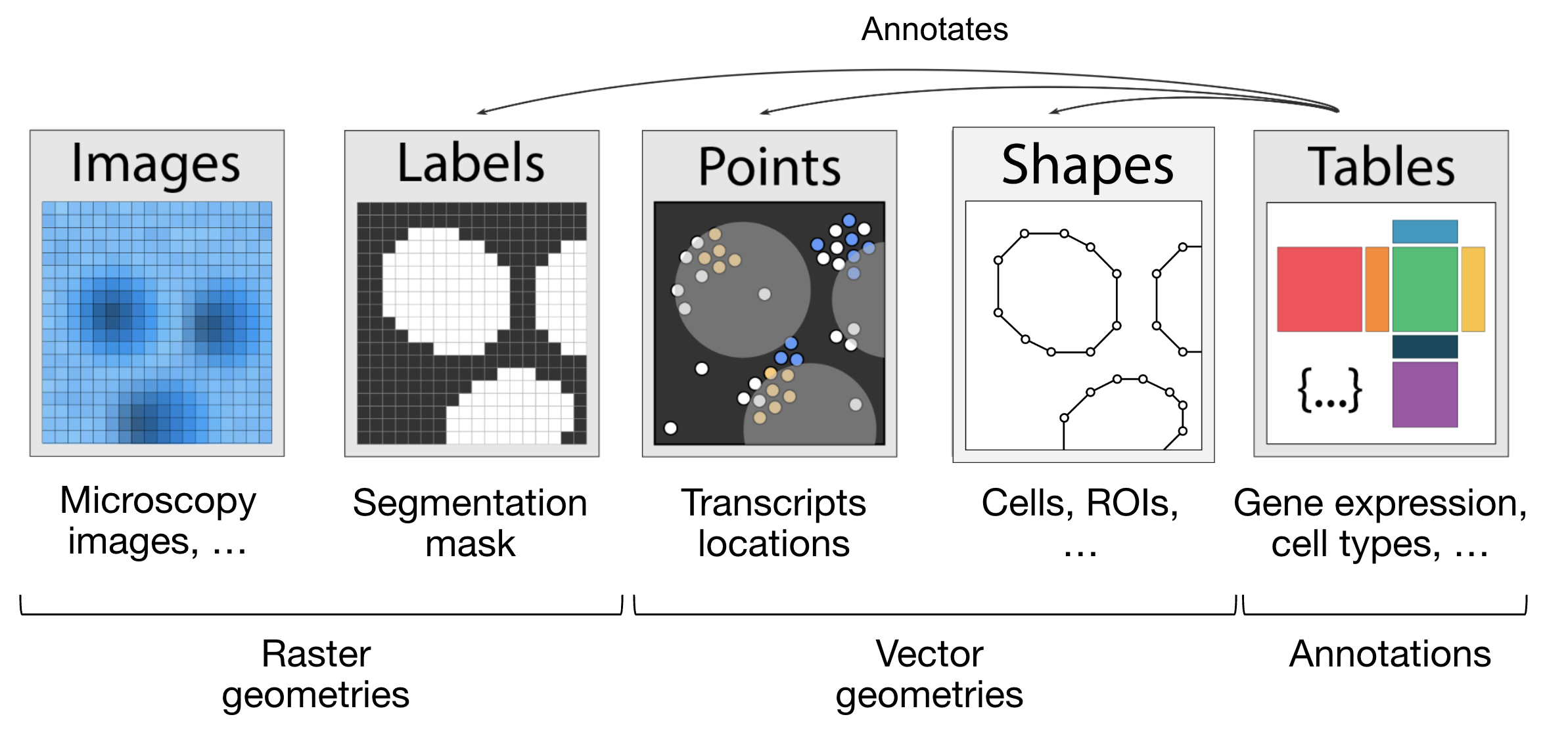
Figure 1:The elements of a SpatialData object. Obtained from Marconato et al., 2025.
import lamindb as ln
import spatialdata as sd
import spatialdata_plot  # noqa: F401

ln.connect("theislab/sc-best-practices")

ln.track("V5rbUBUZEjHh")
Output
→ connected lamindb: theislab/sc-best-practices
! It looks like you are running jupyter lab but don't have jupyter-server module installed. Please install it via pip install jupyter-server
→ loaded Transform('V5rbUBUZEjHh0000', key='data_structures.ipynb'), started new Run('XiKhNtBdq2vjriDz') at 2026-10-19 13:23:19 UTC
Let’s load a mouse liver dataset using lamindb. The original dataset is available here.
sdata = ln.Artifact.get(
    key="introduction/advanced_data_structures_and_frameworks_spatialdata.zarr"
).load()
sdata
SpatialData object, with associated Zarr store: /home/lheumos/.cache/lamindb/lamin-eu-central-1/VPwcjx3CDAa2/introduction/advanced_data_structures_and_frameworks_spatialdata.zarr
├── Images
│ └── 'raw_image': DataTree[cyx] (1, 6432, 6432), (1, 1608, 1608)
├── Labels
│ └── 'segmentation_mask': DataArray[yx] (6432, 6432)
├── Points
│ └── 'transcripts': DataFrame with shape: (1153548, 3) (2D points)
├── Shapes
│ └── 'nucleus_boundaries': GeoDataFrame shape: (3375, 1) (2D shapes)
└── Tables
└── 'table': AnnData (3375, 99)
with coordinate systems:
▸ 'global', with elements:
raw_image (Images), segmentation_mask (Labels), transcripts (Points), nucleus_boundaries (Shapes)Explore the Elements of the SpatialData object
Let’s explore each element type and how they are represented:
Images:
xarray.DataArrayorxarray.DataTreeobjects respectively for single-scale or multi-scale imagesLabels:
xarray.DataArrayorxarray.DataTreeobjects containing integer codes for different labelsPoints:
dask.DataFrameobjects containing point coordinates, (lazy version ofpandas.DataFrameobjects)Shapes:
geopandas.GeoDataFrameobjects containing geometric objects like polygonsTables:
anndata.AnnDataobjects for tabular data with annotations
sdata["raw_image"]Output
Images can have multiple scales, which are stored in a pyramid for downsampled representations useful for more efficient visualization and analysis.
We can access a single scale using the get_pyramid_levels function, where 0 is the highest resolution, 1 is downsampled by a factor of (usually 2), 2 is downsampled by another factor (usually 2, with respect to the previous scale), etc.
In this case, our image has 2 scales (check out groups of the output from the code cell above). Let’s access the highest resolution image.
sd.get_pyramid_levels(sdata["raw_image"], n=1)Output
To view image properties such as axes and channel names, SpatialData provides some helper functions.
More helper functions can be found in the API page.
The axes x and y represent the two-dimensional plane of the image, while c corresponds to the different channels (e.g., wavelength) within the image.
sd.models.get_axes_names(sdata["raw_image"])('c', 'y', 'x')Here we see that our image only has one channel for DAPI staining (highlights nucleus).
sd.models.get_channel_names(sdata["raw_image"])[0]Let’s use spatialdata-plot to show the image (DAPI staining for nuclei).
sdata.pl.render_images("raw_image", cmap="gray").pl.show()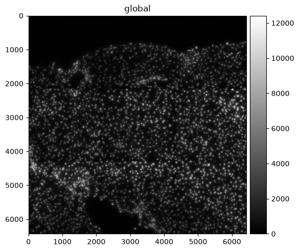
Points
Points are represented as dask.DataFrame objects containing point coordinates (lazy version of pandas.DataFrame objects).
Lazy-loading the DataFrame reduces memory usage, as the information is only retrieved from the data file when it is needed and not all at once.
For spatial transcriptomics datasets measuring single-molecules, coordinates are stored in columns x and y (optionally z for 3D) and have an additional column annotating gene identity.
sdata["transcripts"]We can easily convert the dask.DataFrame to a pandas.DataFrame using .compute() so it is easier to work with.
Note that this will load the entire object into memory.
If the data is large you can use directly the dask APIs for the manipulation of the dataframe.
sdata["transcripts"].compute()When visualizing the points, note that plotting backend automatically switches from matplotlib to datashader.
This ensures performant rendering when the number of points is large.
As you can see below, it will be more useful to plot subsets of transcripts, such as specific genes.
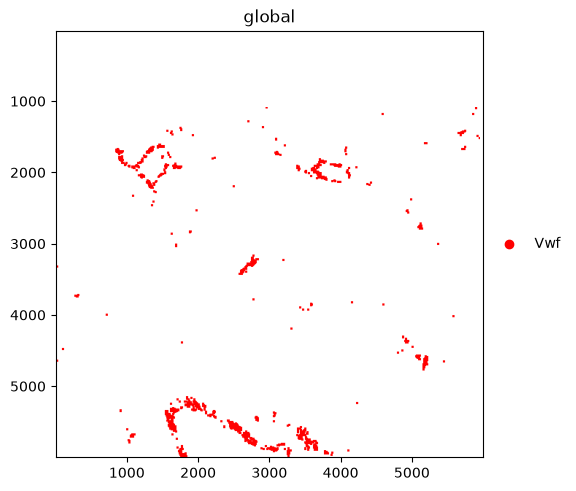
We further plot the transcripts colored by gene.
The groups argument can be used to plot transcripts for a subset of genes.
sdata.pl.render_points("transcripts").pl.show()
sdata.pl.render_points(
    "transcripts", color="gene", groups="Vwf", palette="red"
).pl.show()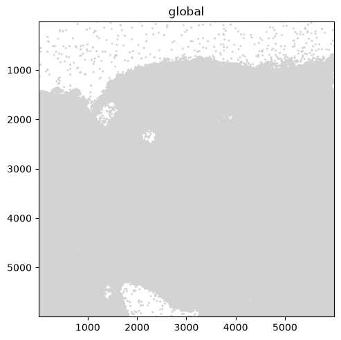
Shapes
Shapes are represented as geopandas.GeoDataFrame objects containing geometric objects like polygons.
For a comprehensive guide on working with geopandas.GeoDataFrame objects, please refer to the geopandas documentation.
sdata["nucleus_boundaries"]sdata.pl.render_shapes("nucleus_boundaries").pl.show()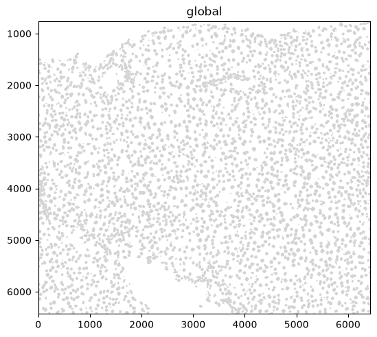
Tables
Annotated matrices are represented as anndata.AnnData objects.
Ingested datasets will usually have a table located at sdata['table'] for a count/abundance matrix.
This enables downstream analysis with tools like Scanpy, scVI, etc.
For different spatial technologies this quantifies:
transcriptomics: transcript counts;
spatial proteomics: marker abundances;
slide-based assays: spot/grid abundances (see spatial chapter).
sdata["table"]Output
AnnData object with n_obs × n_vars = 3375 × 99
    obs: 'cell_ID', 'fov_labels', 'annotation'
    uns: 'annotation_colors', 'spatialdata_attrs'
    obsm: 'spatial'
    layers: None (.X)
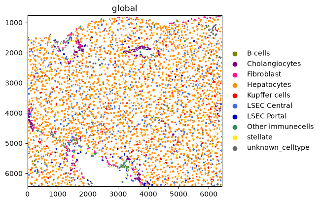
Here is an example of plotting numerical information on the cells (HAL gene expression) and of plotting categorical information (cell types).
sdata.pl.render_shapes("nucleus_boundaries", color="Hal").pl.show()
sdata.pl.render_shapes("nucleus_boundaries", color="annotation").pl.show()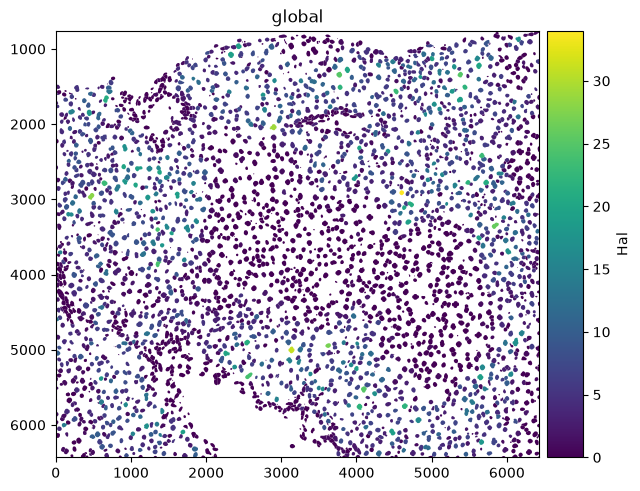
Spatial omics data analysis with Squidpy
Squidpy is a framework to analyze and visualize spatial omics data. It was published around two years before SpatialData Marconato et al., 2025Palla et al., 2022. This is also why Squidpy was originally built on top of Scanpy and AnnData. Squidpy is being updated to work on SpatialData objects directly and to implement the recommendations of the spatial chapters in this book. Until then, most Squidpy functions take the table of a SpatialData object, so this section only gives a short introduction on how Squidpy uses spatial data. Check out future changes and tutorials on the documentation of SpatialData and Squidpy.
API overview
Squidpy’s API lets you analyze and visualize spatial molecular data.
Graph (gr) handles spatial relationships and interactions, image (im) processes and segments tissue images, tools (tl) provides spatial analysis, and plotting (pl) visualizes data and results.
Reading (read) and datasets (datasets) support importing data and example datasets across technologies.
Installation and importing packages
Squidpy is available on PyPI and Conda. It can be installed using either of the following commands.
pip install squidpy
conda install -c conda-forge squidpy
SpatialData integration
Let’s start by importing Squidpy.
import scanpy as sc
import squidpy as sq
We can load a Xenium dataset with lamindb.
sdata = ln.Artifact.get(
    key="introduction/advanced_data_structures_and_frameworks_squidpy.zarr"
).load()
sdata
SpatialData object, with associated Zarr store: /home/lheumos/.cache/lamindb/lamin-eu-central-1/VPwcjx3CDAa2/introduction/advanced_data_structures_and_frameworks_squidpy.zarr
├── Images
│ ├── 'morphology_focus': DataTree[cyx] (1, 25778, 35416), (1, 12889, 17708), (1, 6444, 8854), (1, 3222, 4427), (1, 1611, 2213)
│ └── 'morphology_mip': DataTree[cyx] (1, 25778, 35416), (1, 12889, 17708), (1, 6444, 8854), (1, 3222, 4427), (1, 1611, 2213)
├── Points
│ └── 'transcripts': DataFrame with shape: (42638083, 8) (3D points)
├── Shapes
│ ├── 'cell_boundaries': GeoDataFrame shape: (167780, 1) (2D shapes)
│ └── 'cell_circles': GeoDataFrame shape: (167780, 2) (2D shapes)
└── Tables
└── 'table': AnnData (167780, 313)
with coordinate systems:
▸ 'global', with elements:
morphology_focus (Images), morphology_mip (Images), transcripts (Points), cell_boundaries (Shapes), cell_circles (Shapes)Squidpy demo
Let’s compute a nearest neighbor graph of the spatial coordinates of the xenium dataset.
sq.gr.spatial_neighbors(sdata["table"])INFO Creating graph using `generic` coordinates and `None` transform and `1` libraries.
After that, we can cluster the cells based on gene expression profiles and compute clustering.
%%time
sc.pp.pca(sdata["table"])
sc.pp.neighbors(sdata["table"])
sc.tl.leiden(sdata["table"], flavor="igraph", n_iterations=2)
CPU times: user 53.7 s, sys: 2.66 s, total: 56.3 s
Wall time: 42.7 s
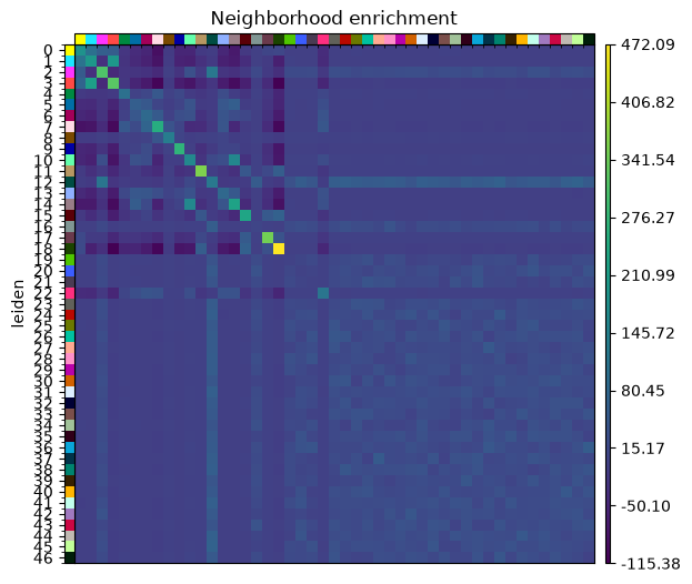
And run the neighbor enrichment analysis in Squidpy.
sq.gr.nhood_enrichment(sdata["table"], cluster_key="leiden")
sq.pl.nhood_enrichment(sdata["table"], cluster_key="leiden", figsize=(5, 5))
100%|██████████| 1000/1000 [00:08<00:00, 115.47/s]
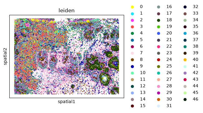
We can finally visualize the results in spatial coordinates both with Squidpy as well as with the novel plotting function in SpatialData.
%%time
sq.pl.spatial_scatter(sdata["table"], shape=None, color="leiden")
WARNING: Please specify a valid `library_id` or set it permanently in `adata.uns['spatial']`
CPU times: user 98.6 ms, sys: 4.98 ms, total: 104 ms
Wall time: 134 ms
Multiple-choice questions
Contributors
We gratefully acknowledge the contributions of:
Authors
Lukas Heumos
Luis Heinzlmeier
Reviewers
Isaac Virshup
- Marconato, L., Palla, G., Yamauchi, K. A., Virshup, I., Heidari, E., Treis, T., Vierdag, W.-M., Toth, M., Stockhaus, S., Shrestha, R. B., Rombaut, B., Pollaris, L., Lehner, L., Vöhringer, H., Kats, I., Saeys, Y., Saka, S. K., Huber, W., Gerstung, M., … Stegle, O. (2025). SpatialData: an open and universal data framework for spatial omics. Nature Methods, 22(1), 58–62. 10.1038/s41592-024-02212-x
- Palla, G., Spitzer, H., Klein, M., Fischer, D., Schaar, A. C., Kuemmerle, L. B., Rybakov, S., Ibarra, I. L., Holmberg, O., Virshup, I., Lotfollahi, M., Richter, S., & Theis, F. J. (2022). Squidpy: a scalable framework for spatial omics analysis. Nature Methods, 19(2), 171–178. 10.1038/s41592-021-01358-2